Mastering Conditional Summation with Excel SUMIFS Function
The SUMIFS function in Excel is a powerful tool used for conditional summation. It allows you to calculate the sum of values in a specified range that meet multiple criteria simultaneously. In other words, it lets you add up values based on certain conditions being satisfied across different columns or ranges.
Here's the basic syntax of the SUMIFS function:
Syntax
=SUMIFS(sum_range, criteria_range1, criteria1, [criteria_range2, criteria2], ...)
- sum_range: The range of cells containing the values you want to sum.
- criteria_range1: The range where you want to apply the first condition.
- criteria1: The condition to apply to criteria_range1.
- [criteria_range2, criteria2], ...: (Optional) Additional pairs of ranges and criteria that you can use to define additional conditions.
The SUMIFS function works by evaluating each cell in the specified criteria ranges against the corresponding criteria. It then adds up the values from the sum range that meet all the specified conditions.
Advantages of Sumif Function
- Conditional Summation: The primary advantage of SUMIFS is its ability to perform conditional summation based on multiple criteria. It allows you to calculate sums selectively, only considering values that meet specific conditions.
- Flexibility: You can apply multiple criteria simultaneously, making the function very flexible. This is particularly useful for complex data analysis scenarios where you need to sum values based on various conditions.
- Simplicity: Despite its power, the SUMIFS function is relatively straightforward to use. Its syntax is easy to understand and implement, especially if you are already familiar with basic Excel functions.
- Dynamic Analysis: SUMIFS enables dynamic analysis of data without the need for manual filtering or sorting. You can change the criteria in your formula to instantly recalculate sums based on different conditions.
- No Extra Columns: Unlike some other methods, SUMIFS doesn't require you to add extra columns to your data for calculations. This helps maintain data integrity and keeps your worksheet organized.
Disadvantages of Sum Function
- Limited to AND Logic: The SUMIFS function uses the AND logic, meaning all specified criteria must be met simultaneously. It doesn't support OR logic directly within the function. To achieve OR logic, you would need to use SUMIFS in combination with other functions or create a more complex formula.
- Complexity for Many Criteria: If you have a large number of criteria or multiple sets of criteria, the SUMIFS function can become complex and hard to manage. In such cases, it might be more efficient to consider other approaches, such as PivotTables or database functions.
- Performance with Large Data: While SUMIFS is generally efficient, it might experience performance issues with very large datasets or numerous calculations involving the function. In such cases, advanced data analysis tools like PivotTables or database management systems could be more suitable.
- Limited to Numeric Data: The SUMIFS function is designed for numeric data. If your criteria involve text or non-numeric values, you might need to use other functions like COUNTIFS or AVERAGEIFS.
- Learning Curve for Multiple Criteria: If you're new to Excel or not familiar with using multiple criteria in functions, there could be a learning curve to effectively utilize the SUMIFS function.
The SUMIFS Function in various ways:
Example 1: Basic Conditional Summation
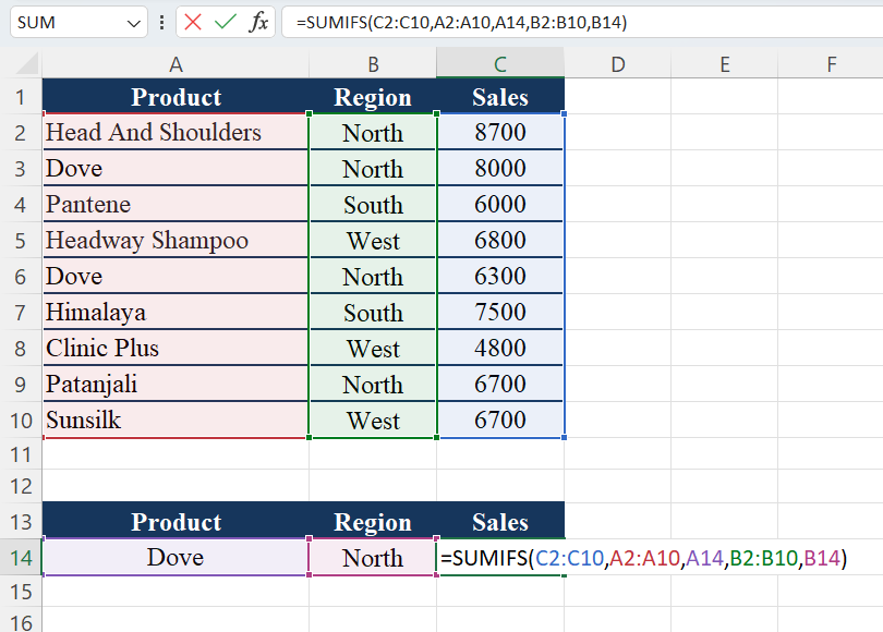
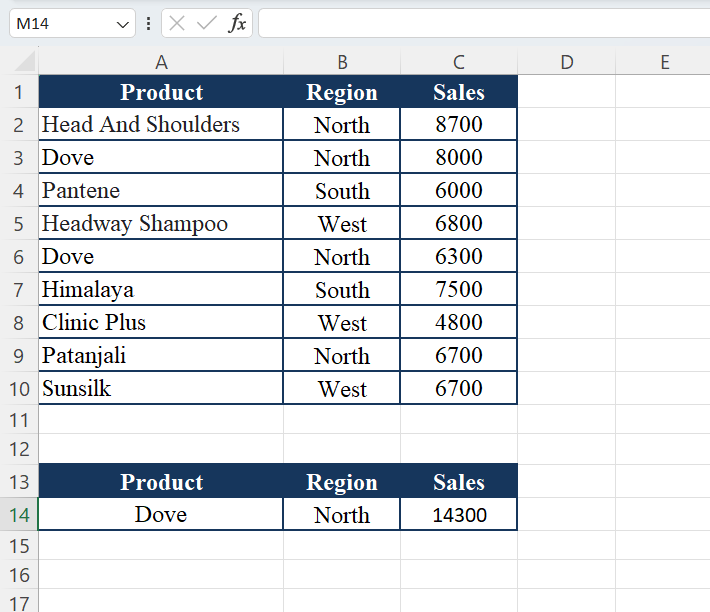
Suppose you have a sales dataset with columns for "Product," "Region," and "Sales Amount." You want to calculate the total sales amount for "Product A" in the "North" region.
Syntax
=SUMIFS(C2:C10,A2:A10,A13,B2:B10,B13)
In this formula:
- C2:C10 is the sum range (Sales Amount).
- A2:A10 is the first criteria range (Product).
- A14 is the first criteria (condition for Product).
- B2:B10 is the second criteria range (Region).
- B14 is the second criteria (condition for Region).
Output
Example 2: Sum of Sales within a Multiple Criteria Ranges
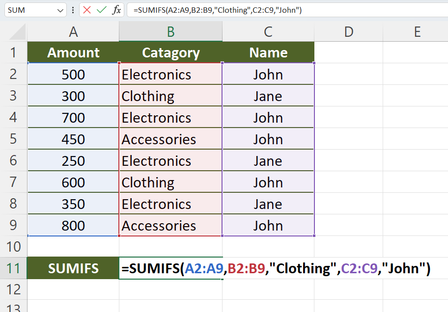
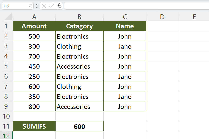
You have a dataset of sales transactions with "Amount," "Category," and "Name" columns. You want to calculate the total sales amount for transactions where the "Category" is "Clothing" and the "Name" is "John."
| Amount | Category | Name |
|---|---|---|
| 500 | Electronics | John |
| 300 | Clothing | Jane |
| 700 | Electronics | John |
| 450 | Accessories | John |
| 250 | Electronics | Jane |
| 600 | Clothing | John |
| 350 | Electronics | Jane |
| 800 | Accessories | John |
Syntax
=SUMIFS(A2:A9, B2:B9, "Clothing", C2:C9, "John")
Explanation:
- A2:A9 represents the range of "Amount" values.
- B2:B9 represents the range of "Category" values..
- "Clothing" is the criteria for the "Category" you're looking for..
- C2:C9 represents the range of "Name" values..
- "John" is the criteria for the "Name" you're looking for..
The formula uses the SUMIFS function to:
- Sum the "Amount" values (column A).
- When the corresponding "Category" value (column B) is "Clothing."
- And when the corresponding "Name" value (column C) is "John."
The function goes through each row of the dataset and includes the "Amount" value in the sum if both conditions are met. In this case, the formula will include the amounts $600 (from the "Clothing" and "John" row) in the sum, resulting in a total sum of $600.
The SUMIFS function is a powerful tool in Excel for calculating sums based on multiple criteria, making it easier to analyze and summarize data from large datasets.
Output
Example 3: Summing Values with Multiple OR Conditions
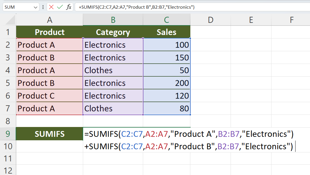
How do I calculate the total sales for "Product A" or "Product B" in the "Electronics" category?
| Product | Category | Sales |
|---|---|---|
| Product A | Electronics | 100 |
| Product B | Electronics | 150 |
| Product A | Clothes | 50 |
| Product B | Electronics | 200 |
| Product C | Electronics | 120 |
| Product A | Clothes | 80 |
Formula
=SUMIFS(C2:C40, A2:A40, "Product A", B2:B40, "Electronics") + SUMIFS(C2:C40, A2:A40, "Product B", B2:B40, "Electronics")
Breaking down the formula using the example data:
- First SUMIFS:
- It sums the sales values (column C) where the product name (column A) is "Product A" and the category (column B) is "Electronics".
- In this example, it sums: $100 (row 1) and $200 (row 4), which gives a total of $300.
- Second SUMIFS:
- It sums the sales values (column C) where the product name (column A) is "Product B" and the category (column B) is "Electronics".
- In this example, it sums: $150 (row 2), which gives a total of $150.
- Adding the results of the two SUMIFS functions:
- $300 + $150 = $450
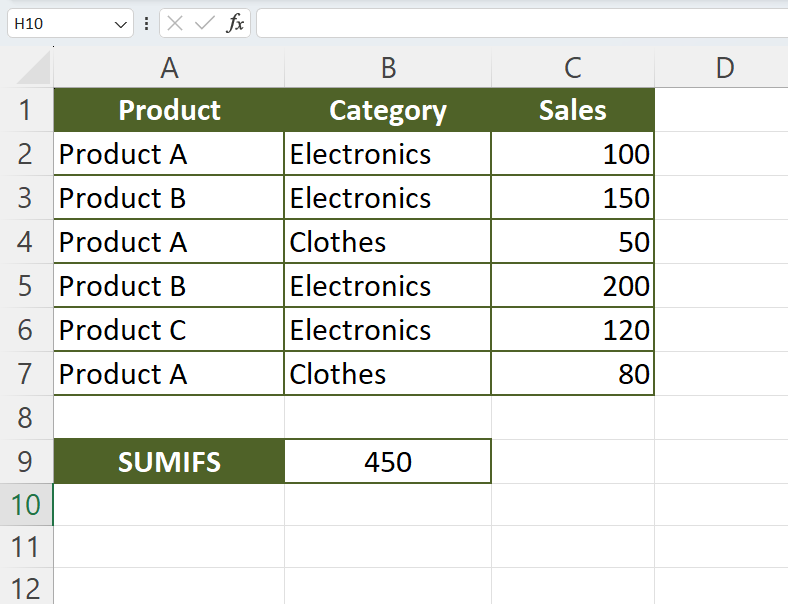
The total sales for "Product A" or "Product B" in the "Electronics" category would be $450 based on the provided example data and formula.
Output
Learn All in Tamil © Designed & Developed By Tutor Joes | Privacy Policy | Terms & Conditions